Previously we used regression to find the best fit line for our data so that we can predict continuous outcomes. If we were to use linear regression on a dataset in Fig. 1 we would not get a model of the data that will allow us to accurately make predictions. Logistic regression uses a logistic function, commonly known as the sigmoid function, to classify data; The sigmoid function better fits binary data.

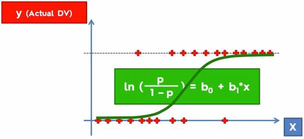Fig. 1. Plot that shows some data with outputs (0 along the x axis and 1 along the dotted lines) and a sigmoid function in green.

As an example fig. 1 is what actual data would look like; we have the independent variable, x, and the output y. Consider the example below:

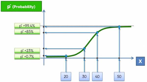Fig. 2. Plot that imposes the data onto the sigmoid function.

In this example, let's say that we want to classify whether or not a banana is genetically modified based on its length (in mm). So the length of the banana is the independent variable (x) and the classification (GMO or not GMO) is the dependent variable (y). Initially the data would look like Fig. 1, but now we are imposing the data onto the sigmoid function based on their values of x. Mapping the data onto the sigmoid function gives corresponding probabilities for the points and those probabilities are how the machine classifies the data. If the probability is less than 50% then the banana is not GMO and if it is greater than 50% then the banana is GMO.

Here is what the python implementation would look like (Does not include importing the dataset, splitting the dataset, and feature scaling): 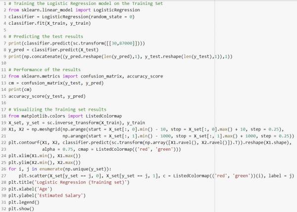Fig. 3. Python Implementation for classification using logistic regression.

In this example the machine is trying to predict whether or not a person will predict a product based on that person's age and salary.

The accuracy of the given classification implementation in python is 89% and a visualization of the performance of the model is shown below: 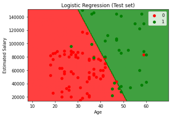Fig. 4. Visualization of the test results from the classification model where red represents the person not buying the product and green represents the opposite.

K Nearest Neighbors is a classification algorithm that classifies points based on the Euclidean distance. The algorithm looks like this:

1. Choose the number, K, of neighbors
2. Take the K nearest neighbors of the new data point, according to the Euclidean distance
3. Among these K neighbors, count the number of data points in each category
4. Assign the new data point to the category where you counted the most neighbors

Looking at an example. Fig. 5 below shows a training set with the red cluster of points being “Category 1” and the green cluster of points being “Category 2”. Let's say we are now trying to determine which category that a new data point belongs to (shown in grey). 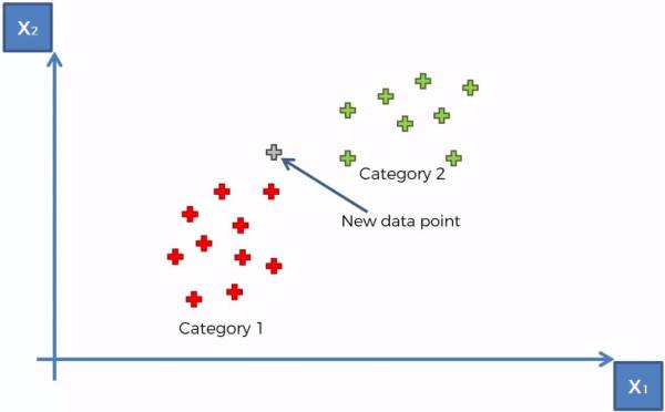Fig. 5. K-NN example with 2 categories and 1 uncategorized data point.

At this point the K-NN algorithm runs (with K = 5) and the 5 closest points are selected. The category with a larger number of points determines what category that the point belongs to. The 5 closest points are shown in Fig. 6 below and we can conclude that the point belongs to Category 1. 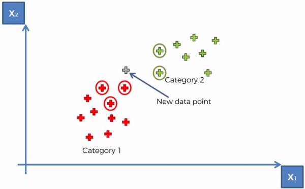Fig. 6. K-NN example showing K = 5 closest neighbors.

The Python implementation of the K-NN classification method is shown (Does not include importing the dataset, splitting the dataset, and feature scaling): 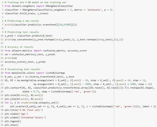Fig. 7. K-NN Python implementation.

This implementation yields 93% and a visualization of the test results is shown: 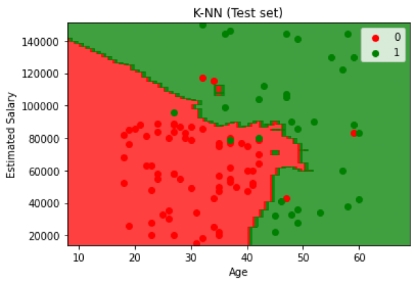Fig. 8. K-NN Test results.

A Support Vector Machine (Sometimes called Optimum Margin Classifier) is another method used to solve the classification problem on datasets. Let's start with an example. Let's say we have two categories shown below as red and green in Fig. 9 (the identities of these categories are arbitrary for now).

Fig. 9. Plot showing two categories within a dataset.

The goal of the SVM is to create an optimum margin between the two groups. We could draw an infinite number of straight lines between the groups to fulfill the goal of simply separating the categories. This is shown in Fig. 10.

Fig. 10. Plot showing some lines that would separate the two groups.

Although there are an infinite number of ways to separate the groups and create a margin, how do we create the optimum margin? The answer is through SVM. The steps for SVM goes as follows:

1. Group the categories and form a convex hull around them (Shown in Fig. 11)
2. Find the shortest line segment that connects the two hulls
3. Find the midpoint of the line segment
4. Draw a line (located at the midpoint of the line segment) that is perpendicular to the line segment
5. This is the optimal hyperplane (Shown in Fig. 12)

Fig. 11. Grouping the categories together to form a convex hull.

Fig. 12. Drawing the optimal hyperplane for SVM.

The implementation for SVM in python is as follows (Does not include importing the dataset, splitting the dataset, and feature scaling):

Fig. 13. Python implementation for SVM (An actual implementation would need, but does not include, data preprocessing).

The classification problem using Support Vector Machines yields a 90% accuracy and the results are shown in the following graph.

Fig. 14. Test set results for classification using Support Vector Machines.

What happens when sets of data aren't linearly separable? Consider the data in fig. 15.

Fig. 15. Single dimension dataset with two categories.

Obviously we can't separate the data with a single line so what do we do? What we can do is map the data onto a higher dimension. Since we're in a single dimension, we have to map the data to two dimensions that will allow us to separate the data. If we mapped the data onto a linear line the data still won't be linearly separable so let's try mapping the data onto a parabola:

Fig. 16. Mapping the data onto a parabola.

Now we can see that we can separate the data with a line:

Fig. 17. Separating the data with a line.

At this point now we map the data and our optimal margin back into the original space. What does this look like in a higher dimension? Consider the data in Fig. 18.

Fig. 18. 2-dimensional dataset with two categories.

Projecting the data into a higher dimension brings us into a third dimension. The data can't be separated by a line in the third dimension but rather a hyperplane. Mapping the data onto a higher space and separating them with the plane is shown in fig. 19.

Fig. 19 Mapping the data into the third dimension and separating the data with a hyperplane.

Finally after separating the data with the optimal margin hyperplane, we map it back into the second dimension and get the following result:

Fig. 20 Mapping the data and hyperplane back onto the second dimension

Mapping to a higher dimension is extremely computationally intensive. Typically data is in a 2D space so most of the time the machine will have to map data into the third dimension. Not only is the computer mapping onto a third dimension but it needs to calculate the optimal margin in 3D space for a hyperplane. With large datasets and complex problems this can take a lot of processing power. So a solution to this is called The Kernel Trick

The Kernel Trick essentially achieves the same goal that mapping to a higher dimension does. There are many kernels to choose from but let's consider the Gaussian RBF Kernel. The equation along with the plot of the Kernel, visualized in 3D, as a function of x and l are shown.

Fig. 21. Gaussian RBF Kernel with K graphed against x, and y

x is the location of some data point and l is the landmark, or center, of the kernel. Note that this Kernel would work with 1-dimensional data as well; K would still be a function of x and l but the visualization would have the data on a 1D line while the visualization of the Kernel is K vs x.

What's happening with the equation is that we're calculating the distance between the landmark and points in our dataset and then adjusting sigma to fit an optimal margin. Sigma controls the base of the RBF function and the base gets mapped onto the dataset which forms the margin that separates the data. Let's consider dataset in Fig. 18 again. To do the kernel trick first we have to set the position of the landmark and then applying the kernel. A visual of this is shown in Fig. 22; We can see that the base of the kernel is mapped onto the 2D space and this is the separation between the categories.

Fig. 22. Applying the Gaussian RBF Kernel onto the data.

As mentioned before, sigma controls the size of the base, which in turn controls how large our margin is. Just like in SVM we adjust the margin, which is sigma, to be the maximum margin, so the maximum distance between the two categories. For some intuition if we increased sigma, we'd have a larger base and thus a larger circle in this example. If we decreased sigma, we'd have a smaller base and thus a smaller circle. Larger and smaller sigma are shown in Fig. 23 and Fig. 24, respectively.

Fig. 23. Graph that provides intuition for a larger sigma.

Fig. 24. Graph that provides intuition for a smaller sigma.

After the machine has trained the model on the training set and found the optimal margin, we have effectively separated the categories. Therefore, when predicting or categorizing new data we simply apply the kernel to the data point and calculate for K. If K is outside of the margin then we can set it to 0 and if it is in the margin then we can set it to K > 0.

Recall that the problem with mapping to a higher dimension was computationally intensive because we needed to map each 2D data point into 3D space and then find the optimal hyperplane in the 3D space and finally map everything back to the 2D space. With the kernel trick, none of the data is mapped onto a higher dimension. Recall the Gaussian RBF Kernel shown in Fig. 21; the kernel is shown in 3D to visualize the energy of the kernel within the margin. Everything that is outside of margin is considered to have K = 0, which means that every point that results in k = 0 belongs to 1 category. With the other category we are simply finding to see if K > 0 and if they are then the point belongs in the other category. The kernel is updated as the margin is adjusted to match the training data. There is no mapping into a third dimension or finding a 3D hyperplane.

The Python implementation for Kernel SVM is as follows (Does not include importing the dataset, splitting the dataset, and feature scaling):

Fig. 25. Kernel SVM Python implementation.

This method yielded 93% accuracy and a visualization of the results are shown:

Fig. 26. Kernel SVM Test Set Results.

Contributing authors:

Created by kmacloves on 2020/12/01 02:24.