Authors

Regression is a statistical process used to define a relationship between a continuous output and one or more inputs. In essence, you are trying to figure how one or more independent variables, x1 x2 x3 …, are related to a dependent variable, y = f(x1, x2, x3, …). We do this by solving for the weights (coefficients), w0 w1 w2 …, which define the relationship between x[] and y. Depending on the set of data, we can choose specific regression models that we feel are best suited to the scenario.

Regression methods discussed on this page:

Simple Linear Regression
Multiple Linear Regression
Polynomial Regression
Support Vector Regression
Decision Tree Regression
Random Forest Regression

Form: y = w0 + w1*x1
When to use it: Used when there is only one independent variable whose degree is assumed to be 1
Library used: sklearn.linear_model.LinearRegression
General workflow:

Import LinearRegression library from sklearn.linear_model
Create an instance of the LinearRegression() class
Apply the .fit method to your independent and dependent variables
Apply the .predict method to your regressor to make any predictions about your data

Sample code and output:

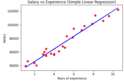
Note that we can easily visualize our results by using a 2D plot. This type of plot is only possible when we have no more than 1 independent variable.

Form: y = w0 + w1*x1 + w2*x2 + … + wn*xn
When to use it: Used when there is more than one independent variable whose degree is assumed to be 1
Library used: sklearn.linear_model.LinearRegression
General workflow:

Use the iloc[rows, columns].values method from the pandas library to grab all columns which correspond to your various independent variables. Note that using iloc[:, :-1].values grabs all rows and all columns except for the last column of your dataset. This assumes that your .csv file was organized such that the dependent variable is in the last column.
Repeat the previous step for your dependent variable using y = dataset.iloc.[:, -1].values
Import LinearRegression class from sklearn.linear_model
Create an instance of the LinearRegression() class
Apply the .fit method to your independent and dependent variables
Apply the .predict method to your regressor to make any predictions about your data

Sample Code and Output:

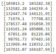
Note that we sometimes cannot create a plot for Multiple Linear Regression because we may have more than 2 independent variables (ie: the graph would have more than 3 dimensions). In this case, we can visualize our results by just printing the predicted output and true output side-by-side in a matrix

Form: y = w0 + w1*x1^1 + w2*x1^2 + w3*x1^3… + wn*x1^n
When to use it: Used when there is only one independent variable whose degree is assumed to be greater 1
Library used: sklearn.preprocessing.PolynomialFeatures
General workflow:

Use the iloc[rows, columns].values method from the pandas library to grab all columns which correspond to your various independent variables. Note that using iloc[:, :-1].values grabs all rows and all columns except for the last column of your dataset. This assumes that your .csv file was organized such that the dependent variable is in the last column.
Repeat the previous step for your dependent variable using y = dataset.iloc.[:, -1].values
Import LinearRegression class from sklearn.linear_model
Create an instance of the LinearRegression() class
Import PolynomialFeatures class from sklearn.preprocessing
Create an instance of the PolynomialFeatures() class and define the degree of your polynomial
Apply the PolynomialFeatures().fit_transform method to your independent variable to change it into a polynomial matrix and save this into a new variable.
Apply the LinearRegression().fit method to your polynomial independent variable and your dependent variable
Apply the .predict method to your regressor to make any predictions about your data

Sample Code and Output: 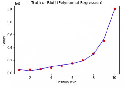Note that we can easily visualize our results by using a 2D plot. This type of plot is only possible when we have no more than 1 independent variable.

Form: Universal. Can be used with any form. Just need to adjust the SVM Kernel accordingly.
When to use it: Used when you want to create an “insensitive tube” (aka noise margin) that cancels out any possible flawed data points due to noise.
Library used: sklearn.SVM.svr
General workflow:

Use the iloc[rows, columns].values method from the pandas library to grab all columns which correspond to your various independent variables. Note that using iloc[:, :-1].values grabs all rows and all columns except for the last column of your dataset. This assumes that your .csv file was organized such that the dependent variable is in the last column.
Repeat the previous step for your dependent variable using y = dataset.iloc.[:, -1].values
Import StandardScaler class from sklearn.preprocessing
Create an 2 instances of the StandardScaler() class, one for your independent matrix, and one for your dependent matrix
Apply the StandardScaler().fit_transform method to your independent and dependent variables to perform feature scaling accordingly
Import SVR class from sklearn.svm
Create an instance of the SVR() class and set your kernel to whatever you want (Radial Basis Function is commonly used)
Apply the SVR().fit method to your independent variable and your dependent variable

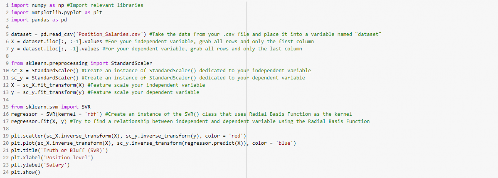
Sample Code and Output: 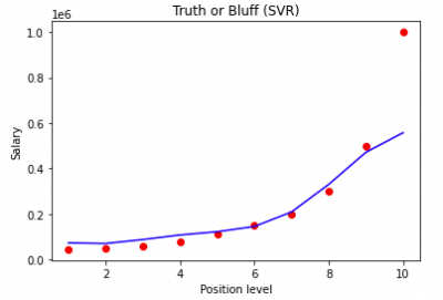Note that we can easily visualize our results by using a 2D plot. This type of plot is only possible when we have no more than 1 independent variable.

Form: Universal. Can be used with any form.
When to use it: Used when you want to divide your dataset into smaller subs-sets in the form of a tree structure
Library used: sklearn.tree.DecisionTreeRegressor
General workflow:

Import DecisionTreeRegressor class from sklearn.tree
Create an instance of the DecisionTreeRegressor() class
Apply the .fit method to your independent and dependent variables
Apply the .predict method to your regressor to make any predictions about your data

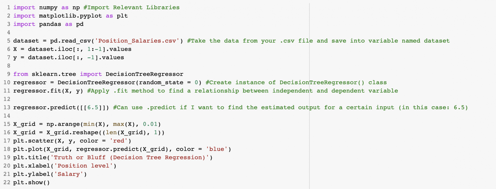
Sample Code and Output: 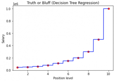Note that we can easily visualize our results by using a 2D plot. This type of plot is only possible when we have no more than 1 independent variable.

Form: Universal. Can be used with any form.
When to use it: Used when you want to have multiple random decision trees to improve your regression results.
Library used: sklearn.ensemble.RandomForestRegressor
General workflow:

Import RandomForestRegressor class from sklearn.ensemble
Create an instance of the RandomForestRegressor() class
Apply the .fit method to your independent and dependent variables
Apply the .predict method to your regressor to make any predictions about your data

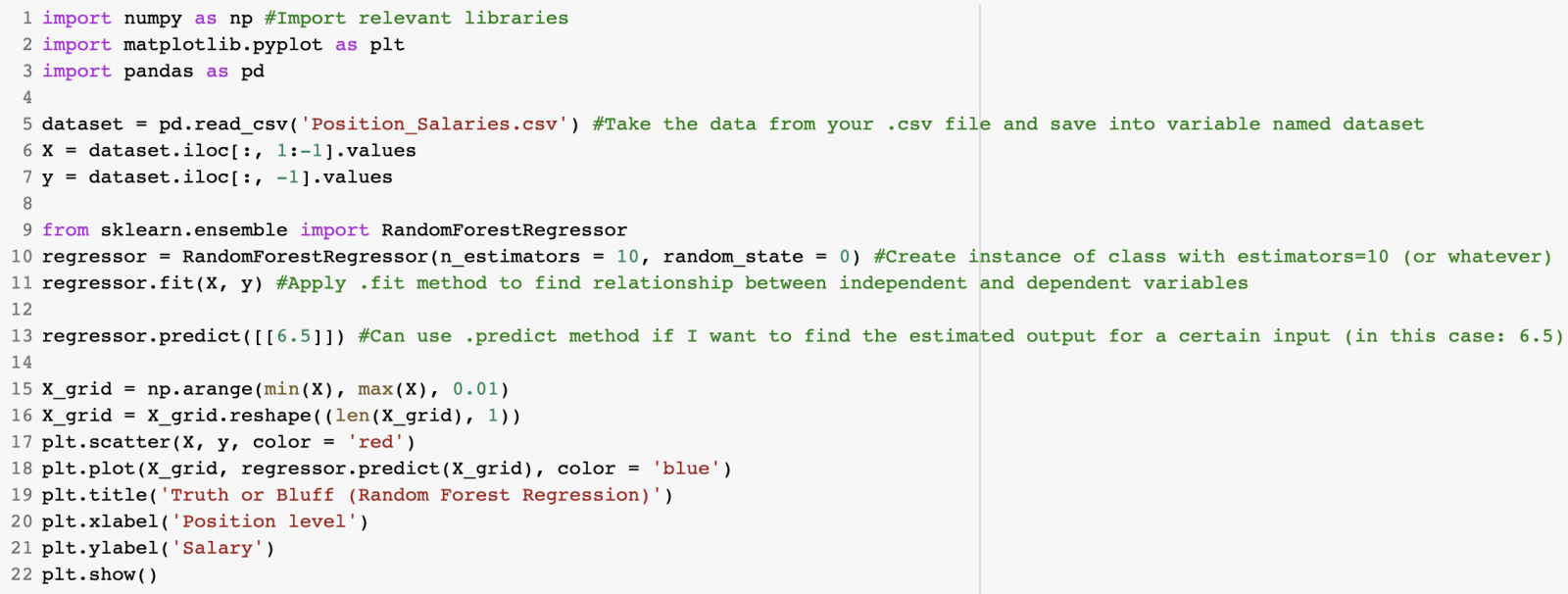
Sample Code and Output: 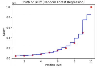Note that we can easily visualize our results by using a 2D plot. This type of plot is only possible when we have no more than 1 independent variable.