Preprocessing the Data
After testing the Wind Sensor, we varied a parameter and took a minute worth of data per trial. After collecting this data, we can create a tall n×m matrix where n is the number of samples and m is different increments of the varied parameter. Lets call this varied parameter x, regardless if it is angle, wind speed or some new parameter. Matlab won't except the reshape function unless it is a rectangular matrix, so chop off any access data on the excel to avoid any errors due to element operands on 'Na' and ensure the fact the all the columns are equal in length. On the top of the data, you should label the column with the ideal value, in this case we will call this vector y. Our matrix is going to be set up as the following,
| y1 | y2 | … | ym |
|---|---|---|---|
| x1,1 | x2,1 | … | xm,1 |
| x1,2 | x2,2 | … | xm,2 |
| … | … | … | … |
| x1,n | x2,n | … | xm,n |
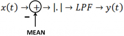
Sound is known to be a sinusoidal wave. Sensors however gives outputs certain ranges. In our case between 0 and 1023. You could take the maximum of this signal and use that to correlate with the y, but it'll only show peaks instead of troughs. Also due to noise(both static and literal) you may get a sharp peak at in a Δt which is independent of y. To avoid this, we subtract the data by the mean (Should be around 1023/2) and take the absolute value so the peaks and troughs are taken into account.
The profits from this is it creates a DC value that is correlated with the amplitude of the sinusoidal signal.
- Note, subtracting the mean of a signal takes away X(0) in the frequency domain.
- squaring a function in time {x(t) → x(t)2} is convolution in frequency domain {X(f) → X(f)∗X(f)}. Also, sound is a real base band signal, so there for it is a low passed signal which is symmetrical around 0. (Squaring is similar to taking the absolute value. Either method could work)
- A convolution between the same signal will be symmetrical and have it's peak in the middle. In this case it is at 0, and X(0) is the DC part which is the total energy in the signal.
- You can find the frequency scaling depending on your sampling frequency. If sampling frequency is ωs, the frequency vector for the fft would go from -ωs/2 to ωs/2.
ProcData = abs(X-ones(size(X,1),1)*mean(X))


From here you could pass it through a LPF (low pass filter Π(f/F)) and take the max, which any random noisy peaks would disappear or get smaller from the low pass filter, you could also take the mean of all of the peaks which will take consideration for all the peaks or you could take the LowestPF (d(f)) and simply take the mean which would take every point into consideration. In this case we took the mean. Now you have a vector of what the sensor has processed size 1×m, let's call it our new X and our Y which was a vector size 1xm.
Correlating the Data
There are many different algorithms to correlate a set of inputs to a set of outputs. In this case we are using linear regression and correlating our X to our Y. {For explanations why this works, things you must be more careful of and other algorithms visit the Forecasting page which_may_or_may_not_be_working}.
You can pick your features (variables on what you are predicting on) For angles, we chose our input X, arccos(X), arcsin(X), arccos(X)arcsin(X) and the y-intercept. For wind-speed, we chose to just use powers of the wind speed.
- For angles, we dropped any values with low correlation/p-values.
- Treated any residual-errors as Gaussian noise which is an assumption needed for linear regression. (For our case this is ok)
- We noticed that you could easily predict Y to X but not X to Y on the wind-speed data.
- We noted that the output graph looked like a square root function, and after squaring, it looked like a linear line,so we predicted on the square of the output, and then we will square root the prediction.
  % For actual fitting you could use either the moving average or regular average (CT or RT).
  % We noticed it look like a trig function, so we just used sin and cos to
  % fit it.

  %Since we our going from output to angle, instead of angle to output, we
  %can't make an explicit function since trig function is not aninvertible
  %function between 0 and 2pi. This is why we are going to overlap from 0 to
  %pi/2
  theta = mod(theta,360);                        % Degrees are circular, so deg = 360*k + deg
  phi = mod(theta,180);
  phi = (theta>180).*(180-phi)+phi.*(theta<180)+180.*(theta==180);

  figure(4)
  hold on
  scatter(CT,phi,'g')
  plot(CT,pred)
  Label('Compare prediction to actual','peak detector','theta');
  legend('Measured','Predicted')

  %We note we are off at low values, so we decided to do a piecewise
  %prediction, 2 different models between first 4 samples and last samples.
  %Note the 4rth sample happens at output < 13.

  bp = 4;                                                   % Break point is at fourth sample
  model = polyfit(CT(1:bp),Speed(1:bp).^2,1);               % fit a model up to Nth degree till break point
  pred = sqrt(polyval(model,CT(1:bp)));                     % evaluate model with input, then squared
  model = polyfit(CT(bp+1:end),Speed(bp+1:end).^2,1);       % fit a model up to Nth degree after break point
  pred = [pred sqrt(polyval(model,CT(bp+1:end)))];          % evaluate model with input, then squared

  figure(5)
  plot(CT,Speed,CT,pred)
  Label('Compare prediction to actual','peak detector','mph');
  legend('Measured','Predicted');

Note we tampered but not fully explored in the frequency domain. Looking at these angles, or amplitudes in general, as speed gets higher the tone gets higher which means the frequency gets higher. (You could use the Find_peak function needed in EE415)This is shown with the impulses getting shifted outward as amplitudes gets higher.

This symmetrical impulses at frequency -fc and fc, corresponds to the Fourier transform of a cosine. Notice how majority of the weight of the signal has most of its energy and magnitude at this impulse. If you also look closely, it is technically also added with a band passed signal which could be due to the microphone specifications. The impulse could be the sound of the fan, but speculation from using different fans and wind speeds lead us to believe that this impulse is the fundamental frequency of the noise of the wind. If you are low passing and sampling, try to stay above the cut off frequencies and stay way above tolerance of that impulse.
Implementing Code
Because the limitations of arduino code, as you probably saw from sampling, has a clock rate + baud rate. Also the sampling speed is altered slightly due to the fact that there has to be delays between sensor readings. This means not only the data will be sampled slower due to the delay, but it will be down-sampled at a rate of k where k is the amount of mics you have. In the case we have, we have 4 pointing orthogonal to its nearest adjacent neighbor on a 2-dimensional plane. Down-Sampling could cause aliasing which you would like to watch out for. For more accurate results, you could then up-sample by the same rate k (add k-1 samples of 0 amplitude between each sample) and low pass filter to try to recreate the signal. From the frequency graph, we were just enough to clear a down-sampling of 4 to not need to up-sample and LPF (Original Sampling at about 5 KHz (4.8 KHz - 5.3 KHz)).
Just like how we did during the signal processing section, we are going to take the output of the sensor and subtract 511 and take the absolute value. The only thing is that keeping the entire data for an entire minute would be costly in memory, even if we take just a second of data and constantly push the last value and queue the newest, that is still (5000 samples/sec)(1sec)(32 bits/sample) = 160,000 bits! You're technically only getting (5000 samples/sec)/(4 mics) = 1250 samples per mic! If you shorten the stack to any reasonable level, you are not getting enough samples for the peak detector to be accurate or mean anything.
What is needed is a memory-less way to update the mean of the current signal. In this case we do a moving average type of equation. Assume you have a signal of N samples with samples k1 to kN with a mean of μ. If you would only like to take the average of the past N samples, after adding sample kN+1, the average would be (kN+1+Nμ-k1)/N. If the variance of the k's are low and/or the N is high enough, you can treat k1 practically as μ. You can calculate for the new mean, lets call it μ[n+1] = (kn+Nμ[n]-μ[n])/N = μ[n+1] (kn)/N + ( (N-1)μ[n])/N If the signal ends up changing from its original mean to a different value, the steady state of this method will converge to the newer mean. Our implementation is below:
function [Y] = RTprocess(X,N)
%Given the input X which is rxk matrix the real time process output Y of
%the peak detector of the past N samples and plots it.
    %   where n is the moving average mean at sample n. It follows the
    %   equation where nth element in vector Y is u[n], for each m columns
    %   u[n] = (x[n]+u[n-1](N-1)u)/N. if x[n] doesn't vary too long and
    %   N is large, it will take the approximate average of the last N
    %   samples. If the signal is in steady state, this function will
    %   converge to the average of the peak detector.

X = abs(X-ones(size(X,1),1)*mean(X)); % Peak Detector x-> [-u]-> [|. |]-> y

Y = zeros(size(X,1),size(X,2));       % Initialize output

for n = 2:size(X,1)
    Y(n,:) = X(n,:)/N + (N-1)*Y(n-1,:)/N; % u[n] = (x[n]+u[n-1](N-1)u)/N.
    end

plot(Y)                               % plot real time process
title('Varied Input Trials')
xlabel('sample')
ylabel('system output')
end
figure(1);                                  % Plots simulational real time process
RT = RTprocess(X,10000);
legend([num2str(theta(1,:)') ones(size(theta,2),1)*(' degrees')])   %Attatch legend with units

Notice if you don't chose a value N large enough, the output of the mean of the last N samples will very large, an example is shown below.
% Test on how the N parameter makes a difference in find the moving average
clc;clear;close all;                    % clears all

t = 0:1/26000:10;                       % Time vector
x = 5*sqrt(t).*sin(10*t);               % signal with increasing mean
figure(1)
plot(t,x);                              % plot signal
Label('Increasing Amplitude Signal','sec','Amplitude');

figure(2)                               % Plot real time process with varied Ns
RT = RTprocess(x',50000);
title('real time process N = 50000')
figure(3)
RT = RTprocess(x',5000);
title('real time process N = 5000')
figure()
RT = RTprocess(x',500);
title('real time process N = 500')
end


From this, we used the equation we found during the data correlation and fit it with the current output and estimate our wind speed. (Note: the model for features x1,x2,…xn, will output a model vector or [w1 ,w2 ,… wn] where y = (w1)(x1)+(w2)(x2)+…+(wn)(xn). If you use polyfit, with fitted N powers, the model would look like [w1, w2,…., wN, wN+1] and will be fitted as y = (w1)(xN)+(w2)(xN-1)+…+(wN)(x1)+(wN+1). A code below where we implement our code and how often we output is shown below.
Note: We did a piece wise regression at output<13 and output>13 because if you look above, that is when it changes a lot faster, and we rather avoid an extra power as a feature to decrease residual error and just use 2 models for 2 parts of the fitting.
The code for collecting data on Arduino is below. This is for collecting analog data before it is processed. This code collects data from all four microphones with a 1 microsecond delay in between readings. Note that each microphone is only being sampled one-fourth of the time. After releasing the reset button on the Arduino, microphone 1 will always be the first data point.
void setup() {
  Serial.begin(14400);
  analogReference(EXTERNAL);
}

void loop() {

  delayMicroseconds(1);
  int sensorValue1 = analogRead(A0);
  delayMicroseconds(1);
  int sensorValue2 = analogRead(A1);
  delayMicroseconds(1);
  int sensorValue3 = analogRead(A2);
  delayMicroseconds(1);
  int sensorValue4 = analogRead(A3);

  Serial.println(sensorValue1);
  Serial.println(sensorValue2);
  Serial.println(sensorValue3);
  Serial.println(sensorValue4);

}
end
Authors
Contributing authors:
Created by jeremygg on 2015/11/24 23:55.